Deep learning for arabic part-of-speech tagging
Deep learning for arabic part-of-speech tagging
- The problem
- Context ignorance
- Part-of-speech tagging
-
- Sequence modeling and RNNs
- How RNN works
- LSTM and long-term dependencies
- A step-by-step LSTM
-
Building an Arabic part-of-speech tagger
- The dataset
- data preprocessing
- model design
- implementation
- Results
- Moving further
Introduction
In this post, I will explain Long short-term memory network (aka . LSTM) and How it’s used in natural language processing in solving the sequence modeling task while building an Arabic part-of-speech tagger based on Universal Dependancy Tree Bank. This post is part of a series in building a python package for Arabic natural language processing. You can check the previous post here.
The problems
Context ignorance
When working on a text data the context of this text matters and can’t be ignored. In fact, words have different meanings based on the context. If we looked at the task of machine translation. Context really matters here while the classical methods will ignore it.
If we are to write a translation method that takes an English sentence and return it translated into Arabic. The naive approach is to take every word from the original sentence and convert it into the target sentence. This approach will work but it will give no regards to any grammar or context.
Part-of-speech tagging
Part of speech tagging is the task of labeling each word in a sentence with a tag that defines the grammatical tagging or word-category disambiguation of the word in this sentence.
The problem here is to determine the POS tag for a particular instance of a word within a sentence.
This tags can be used to solve more advanced problems in NLP like
- Language Understanding because knowing the tags means helps in obtaining a better understanding of the text as different words can have different meaning based on their location within the sentence.
- Text-to-speech and automated speaking tone control.
Ignoring the context when tagging words will only result in the baseline of acceptance as the approach would tagging each word with the most common tag associated with this word from the training set.
So what we are trying to accomplish here is to overcome this issue and find an approach that doesn’t ignore the context of the data.
Deep learning Approach
Sequence modeling and RNNs
More specifically the issue we are trying to solve known as sequence modeling. Where we are trying to model sequential data like text or sound and learn to model it.
Sequence modeling or Sequence-to-sequence modeling was first introduced by Google Translation Team.
In general, Neural Networks are pattern recognition models which learn and enhance by iterating over the dataset and get better in recognizing patterns within the data.
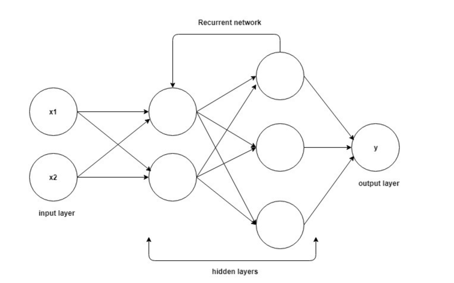
Recurrent Neural Network is designed to prevent neural networks from decay by using feedback loops. Those feedback loops are what makes RNN better at solving the sequence learning task.
RNNs works more similar to a human brain than feedforward networks do. Because the human brain thinks persistently.So, when you are reading this post each word affects your understanding of the post you don’t throw away previous words from your memory to read a new word.
The mechanism of Recurrent neural networks
RNNs address the context of context by using memory units. The output that the RNN produce at step \(N\) is affected by the output from the step \(N -1\). So in general RNN has two sources of input. One is the actual input and two is the context (memory) unit from previous input.
Mathematically,
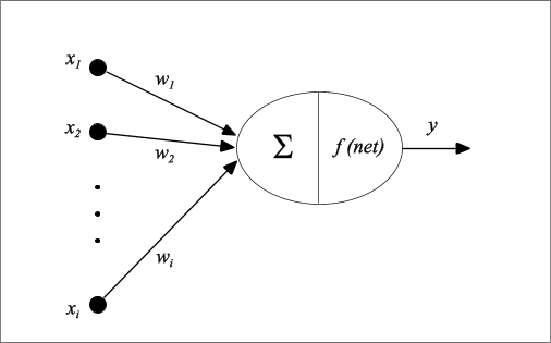
Feedforward networks are defined by the formula \(H_t = F(W * X)\).
The new state is a function of the weights matrix multiplied by the input vector
The result of this multiplication is then passed to the method \(F\) called Activation function. which produce the final result.
The same process is applied in Recurrent network with a simple modification.
\[H_t = F(W * X + U * H_{t-1})\]The previous state \(H_{t-1}\) is first multiplied by a matrix \(U\)
called hidden-state-to-hidden-state matrix then added to the input of the activation function
So \(H_t\) won’t be only affected by \({Xi}\) but all the previous hidden states that has affected \(H_{t-1}\) which will ensure the persistence of memory.
A normal RNN network will contain a single neural network layer which makes it unable to learn to connect long information. This issue is also known as Long-term Dependencies.
Long Short-Term Memory Architecture
RNNs are great. They helped a lot in solving many tasks in NLP. Still they have the issue of Long-Term Dependencies.
you can read more about LTD in Colah’s great blog post here
LSTMs are designed to solve the LTD issue by remembering information for a longer time than RNN.
The only difference between RNN and LSTM that instead having a single neural network layer in RNN. We have 4 NN layers in LSTM interacting together in a special way.
A step-by-step LSTM
An LSTM layer consists of a chain of cell states \(C\) where each state consists of 4 main layers and 3 gates.
Now let’s walk through an LSTM cell state step by step
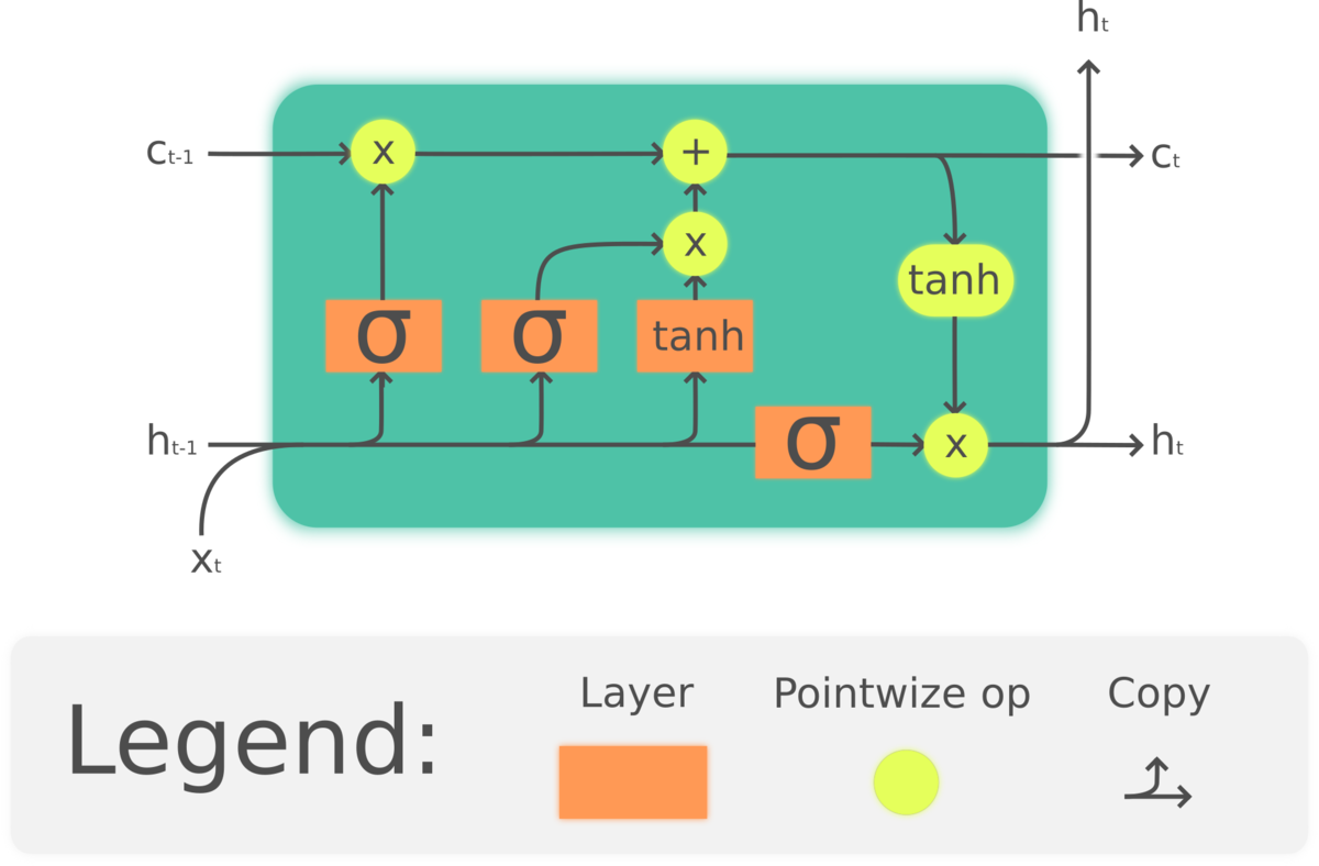
The core of a cell state is the horizontal line that connects between \(C_{t-1}\) and \(C_t\) . This line is where the data flow happens throw the chain of the cell states. It’s very easy for the data to flow with minimum linear operations or unchanged this whole process is controlled by Gates.
Gates are what control the change of the data. They change the data optionally with a sigmoid neural layer \(\sigma\) and a vector mutliplication operation.
The Sigmoid layer is a method that generates float value between \(0\) and \(1\) this value control how much data will be passed through the gate. \(Zero\) means nothing while $One$ means all.
The first step is that the sigmoid layer decide what information to pass from the result of multiplying \(h_{t-1}\) by \(X_t\). We can represent this operation mathematically like this:
\[f_t = \sigma(W * X + H_{t-1})\]The previous step did decide what data it’ll forget and what data it’ll carry on. In the second step, we need to actually do this.
We take the previous result \(f_t\) and multiply it by the old state.
The old state is computed using the Tanh activation function. Multiplying the sigmoid by the tanh will decide which information the network forget and which get. Mathematically:
\[\hat{C_t} = Tanh(W * X + H_{t-1})\] \[C_t = f_t *(\hat{C_t} + C_{t-1})\]Finally we need to decide what is the value of \(H_t\)
\[H_t = f_t * Tanh(C_{t-1})\]Those operations are applied sequentially on the chain of cell states. Looking at the mathematical model of an LSTM can be intimidating so we are going to move to the applied part and implement an LSTM model with Keras for POS-tagger for Arabic language.
Building an Arabic part-of-speech tagger
Know as we walked through the idea behind deep learning approach for sequence modeling. We will apply that to build an Arabic language part-of-speech tagger.
For English language, PoS tagging is an already-solved-problem. For a reach morphological language like Arabic. The problem still persists and there is ZERO open sources deep-learning based Arabic part-of-speech tagger. Our goal know is to use what’ve learned about LSTMs and build an open source tagger.
The data
The lack of open source tagger is an obvious result of the lack of an Arabic treebank dataset.
The well-known Penn Tree Bank costs around 3k$ and the Quranic Tree bank is very classical and perform poorly on day-to-day words.
Universal Dependencies (UD) is a framework for cross-linguistically consistent grammatical annotation and an open community effort with over 200 contributors producing more than 100 treebanks in over 70 languages Including Arabic
UD provides 3 different treebanks. We are going to use the PADT tree bank as suggested by the reviews.
Data Preprocessing
UD provides the data set in CoNLL form. We can use pyconll to convert the dataset from CoNLL format into pandas data frame.
We need our data to be sequentially structured. So we need it in the following shape
[
    [(Word1, T1), (Word2, T2), ...., (WordN, TM)], # Sentence one
    [(Word1, T1), (Word2, T2), ...., (WordN, TM)], # Sentence two
    .
    .
    .
    [(Word1, T1), (Word2, T2), ...., (WordN, TM)] # Sentence M
]
Now as the data set is structured in a usefull way. We want to encdoe our text data to numerical values.
This process is known as WordEmbedding.
The idea is simple, we give each word in our data a unique integer value. And substitute with this value in the data set so we can do pointwise operations on the data.
So before implementing the model we have two WordEmbeddings word2index and tag2index. Which encode the words and the part-of-speech tags
Because we are doing seq2seq task which requires the input and the output to be fixed . The data should be transformed such that each sequence has the same length. This vectorization allows the LSTM model to efficiently perform batch matrix operation.
We can do this in keras by adding 0’s to the shorter sentences until all our sentences have the same lengths.
The problem is that the model will be able to predict those values easily. So the accuracy will be very high even if the model didn’t predict any tag correctly.
So we will need to write our own accuracy metrics that ignores those paddings predictions.
Keras implementation of LSTM
After converting the data to a suitable shape. The next step was to design and implement the actual model.
The model
model structure
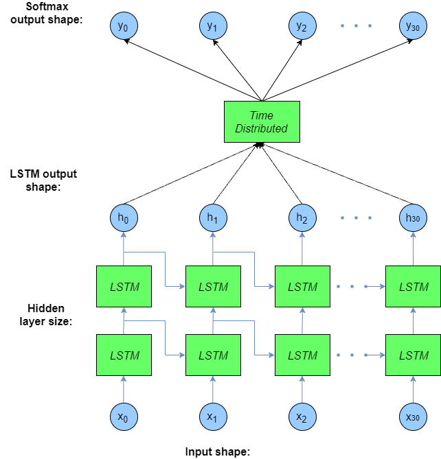
Now let’s explain the model thoroughly,
InputLayer is the first layer of the model. Keras has fixed size layer as explained in the preprocessing part so we define this layer with the maximum length of a sequence in the training set.
Embedding The embedding layer requires that the input data be integer encoded, so that each word is represented by a unique integer. It is intialized with random weights then it will learn for each word in the dataset
LSTM The LSTM encoder layer is a sequence-to-sequence layer. It provides a sequence output rather than an integer value. And return_sequences force the layer to make the previous sequence an input for the next one.
Bidirectional Bidirectional wrapper duplicates the LSTM layer so we habe two side-by-side layers that transfers the resulted sequences to the inputed one. In practical this approach has a great effect on the long short-term memory. I used the default merge mode [concat] for the Bidirectional layer.
TimeDistributed Dense layer is used to keep one-to-one relations on input and output layers. It applies a same Dense (fully-connected) operation to every timestep of a 3D tensor.
Activation The activation method for the Dense layer. We could’ve defined the activation method as a paramater in the Dense layer but the second one is a better approach*
Implementing this design with keras is very straightforward.
model = Sequential()
model.add(InputLayer(input_shape=(MAX_LENGTH, )))
model.add(Embedding(len(word2index), 128))
model.add(Bidirectional(LSTM(256, return_sequences=True)))
model.add(TimeDistributed(Dense(len(tag2index))))
model.add(Activation('softmax'))

model.compile(loss='categorical_crossentropy',
              optimizer=Adam(0.001),
              metrics=['accuracy', ignore_class_accuracy(0)])
model.summary()
We use categorical_crossentropy as a loss function because we have a many-to-many labeling problem.
and Adam optimizer (adaptive moment estimation) for training.
ignore_class_accuracy is a method to recompute accuracy after ignoring the padding <PAD>
Results
The training steps took around 40 mins on a 2017 MacBook Pro with 2.5 GHz CPU and 8 GB Ram.
After we train our model we evalute and visualize the training process it.
model.compile(loss='mean_squared_error',
              optimizer='sgd',
              metrics=['mae', ignore_class_accuracy(0)])
model.evaluate(test_sentences_X, to_categorical(test_tags_y, len(tag2index)))
680/680 [==============================] - 10s 14ms/step
[0.0009350364973001621, 0.0011567071230862947, 0.9160830103105271]
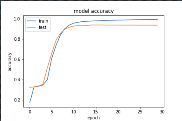
# summarize history for accuracy
plt.plot(history.history['ignore_accuracy'])
plt.plot(history.history['val_ignore_accuracy'])
plt.title('model accuracy')
plt.ylabel('accuracy')
plt.xlabel('epoch')
plt.legend(['train', 'test'], loc='upper left')
plt.show()
# summarize history for loss
plt.plot(history.history['loss'])
plt.plot(history.history['val_loss'])
plt.title('model loss')
plt.ylabel('loss')
plt.xlabel('epoch')
plt.legend(['train', 'test'], loc='upper left')
plt.show()
Model Loss
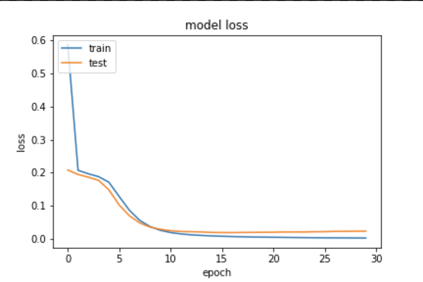
The model has reached 0.916 and started to converge after 30 epochs
In the evaluation we used stochastic gradient descnet as it perform better than Adam in the evaluation*
Despite the results looks good comparing to stanford corenlp model yet it can be enhanced. But as a first try it’s not bad.
The whole source code is in the the project repository: https://github.com/adhaamehab/arabicnlp
References
- https://shaoanlu.wordpress.com/2017/05/29/sgd-all-which-one-is-the-best-optimizer-dogs-vs-cats-toy-experiment/
- https://machinelearningmastery.com/data-preparation-variable-length-input-sequences-sequence-prediction/
- http://colah.github.io/posts/2015-08-Understanding-LSTMs/
- https://skymind.ai/wiki/lstm
- https://kevinzakka.github.io/2017/07/20/rnn/
- https://developer.nvidia.com/discover/lstm
- https://iamtrask.github.io/2015/11/15/anyone-can-code-lstm/
- http://karpathy.github.io/2015/05/21/rnn-effectiveness/
- https://universaldependencies.org/